![[0x0v1]](https://www.0x0v1.com/content/images/2023/09/0x0v1-1.png)


The visualization of malware has been a widely discussed topic over the years, though it hasn't garnered as much attention in the last decade. Nearly ten years ago, infosec experts like Chris Domas (TED talk linked below) highlighted the potential of malware visualization as a powerful tool for analysts to quickly and effectively understand malware. These efforts likely made significant impacts in cybersecurity, evidenced by the adoption of some of the tools discussed back then in various cybersecurity platforms.
These principles essentially use digraphs, short for "directed graphs," a concept from graph theory, which is a branch of discrete mathematics. In a digraph, the connections between nodes (also called vertices) are directional, meaning they go from one node to another specific node. There are various methods for converting binary data into plots to understand the connections between nodes. Once plotted, these connections can be visually represented and further analyzed using additional algorithms or systems.
While I find binary visualization for analysis to be an interesting topic, I believe its application is limited. Personally, I think it is much more intriguing to explore it as a mechanism for artistic and exploratory purposes. It allows us to understand complex patterns and particularly allows lay people's the ability to understand these complexities at a high level. Personally, I find these visualizations intricate and aesthetically pleasing. With this, the abstract nature of binary visualization lends itself well to contemporary art forms, in addition to new media art and cross-disciplinary work.
The idea behind this is to allow for conceptual depth to be understood. The representation of data; visualizing binary data transforms the invisible and abstract world of digital information & malware into something tangible and visible. This can create a conceptual bridge between the digital and physical worlds, providing a fresh perspective on how data shapes our reality or as impacted human life. This allows us to explore and comment on the impact of binaries, malwares & softwares in modern life, raising awareness and provoking thought about the digital age.
In this post, I will discuss how to convert binaries into 3D models (represented below). I will demonstrate methodologies to do this & provide free open-source software to support your own developments of this. Finally, I will present some visualizations as part of my instructSOCIETY project, with source files which I have made available for paid subscribers of my website.
In order to first convert a binary into a format which we can plot, we need to take the executable and convert it into a number system. Using hex is the easiest way to do this. In the follow code snippet, we will provide a function that converts binary data of an executable file into a hexadecimal string. It will write this string to an output file which we can process later.
import binascii

def exe_to_hex(input_file, output_hex_file):
    try:
        with open(input_file, 'rb') as exe_file:
            binary_data = exe_file.read()
    except Exception as e:
        print(f"Error reading input file: {e}")
        return

    try:
        hex_data = binascii.hexlify(binary_data).decode('utf-8')
        with open(output_hex_file, 'w') as hex_file:
            hex_file.write(hex_data)
        print(f"Conversion to HEX complete. HEX data written to {output_hex_file}")
    except Exception as e:
        print(f"Error writing to output file: {e}")

# Example usage
# exe_to_hex('input.exe', 'output.hex')
We then need to plot the hex data into coordinates. The best way to do this is by simply using XYZ coordinates. However, since some binaries are extremely large, plotting hex data as XYZ coordinates can result 3D model engines crashing. So we need to offer some opportunity to downsample. This means we can skip hex coordinates to scale it down. Once we offer that, we can process the hex data. We can do this by processing the hex data in chunks of 6 characters (2 characters per coordinate axis: X, Y, Z). It will then convert each chunk into three integers (0-255), representing X, Y, Z coordinates. Once we have our conversion, we'll want to output this file, since we can then apply it to 3D model engines and such.
import os

def hex_to_xyz(input_hex_file, output_xyz_file, downsampling_factor=1):
    """
    Converts hex data from an input file into XYZ coordinates and writes them to an output file.

    Args:
    - input_hex_file (str): Path to the input file containing hex data.
    - output_xyz_file (str): Path to the output file to write XYZ coordinates.
    - downsampling_factor (int): Factor to downsample the data. Must be between 1 and 10.
    """

    if not (1 <= downsampling_factor <= 10):
        print("Invalid downsampling factor. Please choose a value between 1 and 10.")
        return

    try:
        with open(input_hex_file, 'r') as hex_file:
            hex_data = hex_file.read().strip()
    except (FileNotFoundError, IOError) as e:
        print(f"Error reading input HEX file: {e}")
        return

    if len(hex_data) % 6 != 0:
        print("Warning: Hex data length is not a multiple of 6, some data might be incomplete.")

    points = []
    for i in range(0, len(hex_data), 6 * downsampling_factor):
        hex_coord = hex_data[i:i + 6]
        if len(hex_coord) < 6:
            print(f"Skipping incomplete HEX coordinate: {hex_coord}")
            continue

        try:
            x = int(hex_coord[0:2], 16)
            y = int(hex_coord[2:4], 16)
            z = int(hex_coord[4:6], 16)
            points.append((x, y, z))
        except ValueError:
            print(f"Skipping invalid HEX coordinate: {hex_coord}")

    try:
        with open(output_xyz_file, 'w') as xyz_file:
            for point in points:
                xyz_file.write(f"{point[0]} {point[1]} {point[2]}\n")
        print(f"Conversion to XYZ complete. Points written to {output_xyz_file}")
    except (FileNotFoundError, IOError) as e:
        print(f"Error writing to output XYZ file: {e}")

# Example usage
# hex_to_xyz('input.hex', 'output.xyz', downsampling_factor=2)
Once we have an XYZ coordinate file, you can apply this to other algorithms for visualisation. If you're using Blender for 3D modelling, you'll want to create a PLY file though. Polygon File Format files allow for the store three-dimensional data, and will allow us to develop 3D models more easily. So first we need to take an XYZ coordinate file, like the one we previously set up, and read it into our script. We then need to generate a PLY header & then iterate over each line of the XYZ data & convert them into floats, then write them to the PLY file. Here's an example:
def xyz_to_ply(input_xyz_file, output_ply_file):
    try:
        with open(input_xyz_file, 'r') as xyz_file:
            xyz_data = xyz_file.readlines()
    except Exception as e:
        print(f"Error reading input XYZ file: {e}")
        return

    with open(output_ply_file, 'w') as ply_file:
        ply_file.write("ply\n")
        ply_file.write("format ascii 1.0\n")
        ply_file.write(f"element vertex {len(xyz_data)}\n")
        ply_file.write("property float x\n")
        ply_file.write("property float y\n")
        ply_file.write("property float z\n")
        ply_file.write("end_header\n")

        for xyz_line in xyz_data:
            x, y, z = map(float, xyz_line.split())
            ply_file.write(f"{x} {y} {z}\n")

    print(f"Conversion to PLY complete. Points written to {output_ply_file}")
The combined script for this method has been uploaded to my Github account where you can download it for free. This script also includes a number of other useful functions which we can go into later in the blog post.
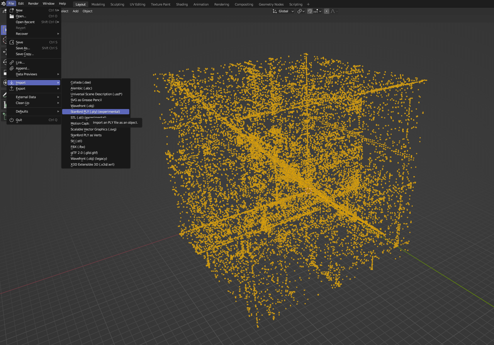
Once we have our PLY file, we're ready to load into Blender to arrange our 3D model. You can of course use whatever modelling software you chose, but here I'll only cover Blender.
With Blender, we can 'import as PLY', which will load our PLY file as a point cloud.
I won't go into the intricacies of Blender here, as you can explore modifying the model yourself (there's plenty of tutorials online about how to customize models). But we're going to create a Geometry Node for our point cloud. In the Scene Collection tab, click your point cloud & then navigate to the Geometry Node section. Create a new Geo & use the following scheme. This will create a cube for each point in the cloud, allow us to set a material (which can be customized), instance the points, realize them and output. You can of course modify this.
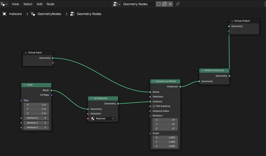
The result will give us a more suitable looking point cloud, which we can then customize to our liking using Blender's 3D modelling suit.
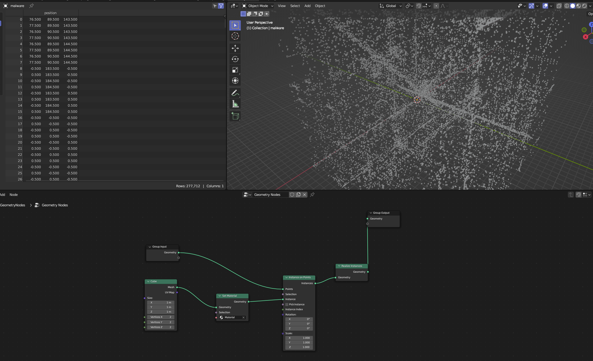
Here's an example of my conversion of RokRAT malware into a pointcloud, this file was relatively small so I didn't have to downsample it. I've then used Blender to create the 3D model, and exported as GLB file, which is then being hosted by Github & rendered by Google's Model Viewer
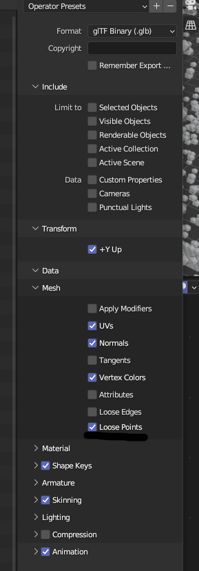
When you wish to export your 3D model, export to .GLB file. In your export settings ensure you select Mesh > Loose Points, otherwise your pointcloud will not render.
Being able to export a GLB file with a 3D model of a binary allows for a multitude of explorations with artistic expression & creatitvity.
In my project instructSOCIETY, I am using 3D models to visualize malware in ways to impact conversation around human rights issues related to nation-state sponsored attacks. In this project, you can demonstrations of 3D modelling such as this, which shows RokRAT malware, plotted using one line with resonance create by CPU load.
Tutorial here
If you wish how to learn to do this, I will discuss this in a subscriber only post here. Subscribers will be able to view the post, download project files and get started doing the same straight away.
 Ovi
Ovi
Doing more with digraphs
If you checked out my instructSOCIETY python script, you will see that there's a secondary tool in there that will allow you to perform some visualizations with your binary data. The options presented in the tool are:
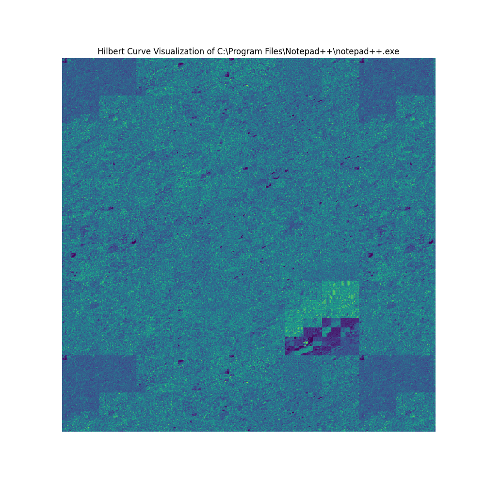
Hilbert curve
The Hilbert curve is a type of space-filling curve discovered by the German mathematician David Hilbert in 1891. It is a continuous fractal curve that visits every point in a square grid with a specified order. This makes it particularly useful for tasks that require spatial locality, such as image processing, data indexing, and other applications such as binary visualization.
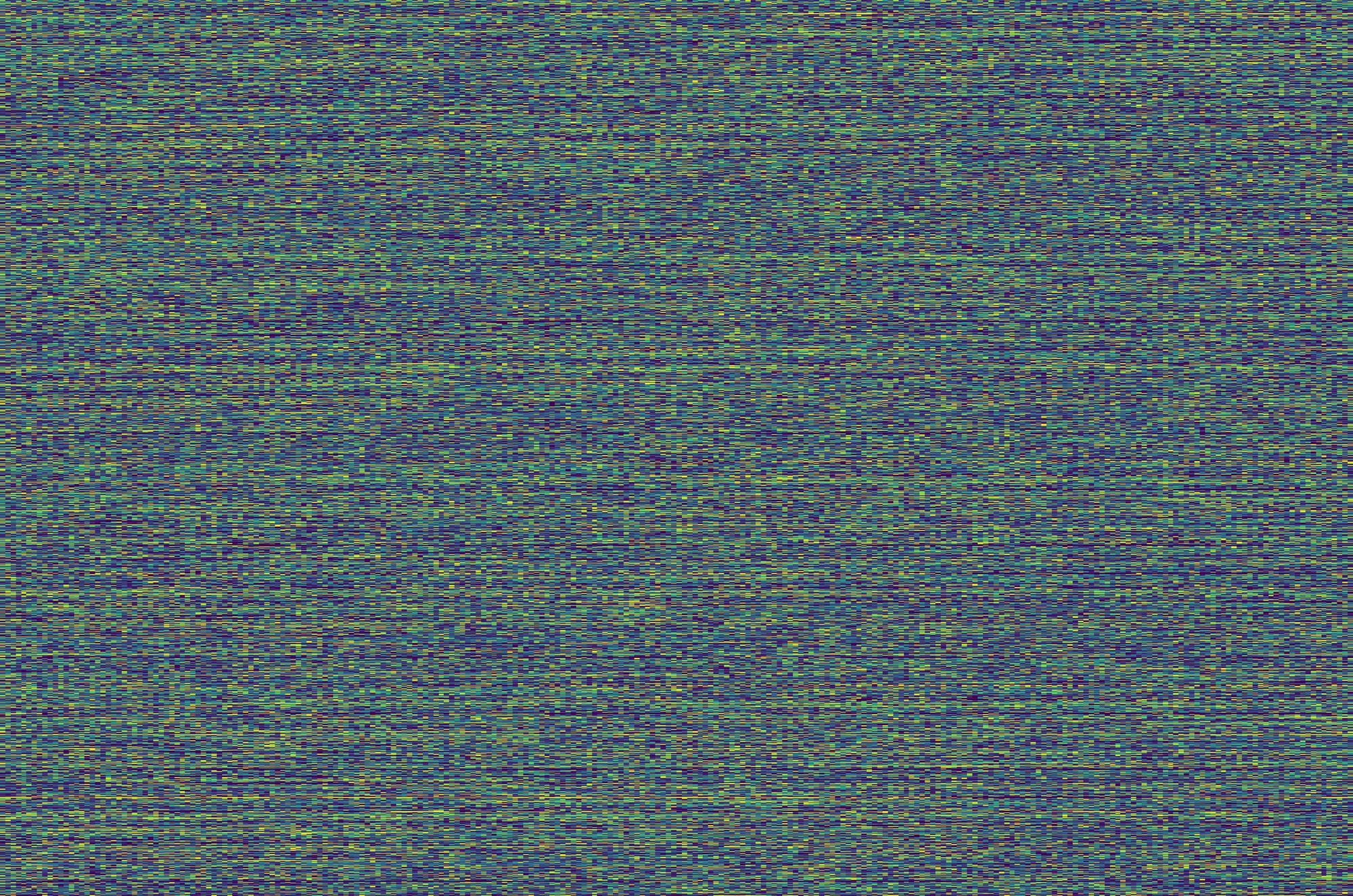
Natural-order traversal
Natural-order traversal is the simplest and most straightforward way to traverse a grid or matrix. It involves visiting each element in a sequential manner, typically row by row or column by column. This type of traversal does not consider any specific curve or path but rather follows the natural arrangement of the elements.
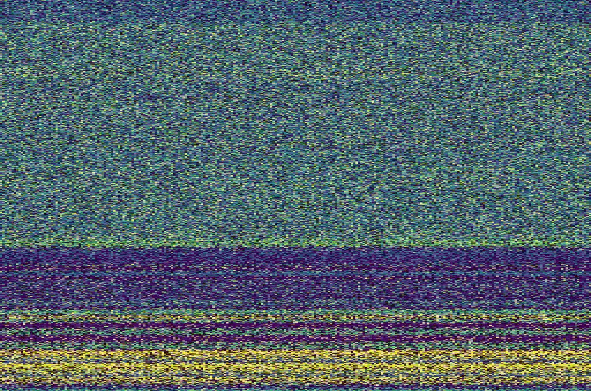
Zigzag traversal
Zigzag traversal is a method of traversing a grid or matrix in a zigzag pattern. It is often used in scenarios where alternating directions provide some benefit, such as reducing the number of abrupt changes in direction, preserving some level of locality, or optimizing specific types of data access patterns.
In the next blog I'll be discussing more visualization techniques and how to incorporate AI methods. To learn how to perform motion plotting and visualization techniques of malware (as seen in the video in this blog), click here for exclusive content which includes project files so you can get started straight away.
instruct.SOCIETY
malware impacting human rights
the g4llery <-